Introducing – Binomial Ranking

From pundits baselessly exclaiming “He’s go to score there” and statisticians struggling to find much repeatability, finishing is a universally difficult skill to asses. A recent sequence of tweets from Michael Caley shows an analysis and ranking of players based on their “Finishing skill” measured in this case by (Goals – Expected goals) per 50 shots. One of the problems he says he faced though is reliability and he seems to have used a cut off of 600 shots in order to compensate and obtain more reliable results (although 600 shots seems pretty high and he may have just regressed players below 600 shots) .

Although G-xG per shot seems like an intuitive way to define finishing skill, one of it’s problems is that it punishes players that have taken more shots, which shouldn’t be the case, especially when players with higher shot totals tend to have better “finishing skill”. Another popular way of measuring finishing skill is to use total G-xG to see which players have added the most goals above expectation. The problem with this method is that it doesn’t take number of shots into account at all, so players with more shots are likely to be given an unfair advantage.

Let’s create a hypothetical situation to picture this better.

Let’s take a made up player called “John Smith”. In his career he’s taken 100 shots, scored 11 goals with an xG of 10. His G-xg is therefore 1 and his G-xG per 50 shots is 0.5.

Now we’ll look at another made up player “Jack Jones”. In his career he’s taken 1000 shots, scored 109 goals with an xG of 100. his G-xG is 9 and his G-xG per 50 shots is 0.45, less than that of John Smith, so by the G-xG per 50 shots method John Smith is the better finisher. But Jack Jones has taken waaaay more shots (1000 to 100) so his finishing skill data is much more reliable and he’s also added more goals than expected (9 to 1) so there’s definitely reason to argue that Jones is the better finisher.

There is a way we can fairly test finishing skill, taking into account number of shots but not punishing players for it.

We can consider each shot to be a Bernoulli Trial with a probability “p” of success (a goal) and probability “q” of a failure (no goal). Now if we have “n” number of shots we have a Binomial experiment where each shot has probability “p” of success and “q” failure. The problem with this is that not every shot has the same probability of success, but we can create some Monte Carlo simulations to test whether the binomial probabilities (using the average xG value as “p”) follow the true success rate. But first I’ll go through the methodology of the binomial ranking.

For a player with x goals in n shots, we want to work out the probability that an average player would have got less than x goals in n shots. To do this we can calculate the cumulative probability of less than or equal to x goals using the excel function =BINOM.DIST(Goals,Shots,xG/Shots,TRUE) then minus the probability of exactly x goals =BINOM.DIST(Goals,Shots,xG/Shots,FALSE). The higher the probability the better that particular player is at finishing.

Let’s use Monte Carlo simulations to test whether the binomial distribution is appropriate. I didn’t have any data on the spread of expected goals but found a distribution that I thought worked pretty well. I modeled the success rate of a shot by {Rand()*Rand()*Rand()} where Rand() is a random number between 0 and 1. I found that this distribution has a mean of 0.125, which is  close to an average strikers conversion rate. About 40-45% of these shots have an xG of <0.05 which holds up well with 42% of premier league shots being taken outside the box. Also about 6-7% of these shots have an xG of  >0.4 which seems about right considering about 12% of shots are big chances.

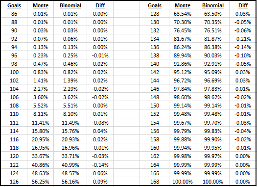
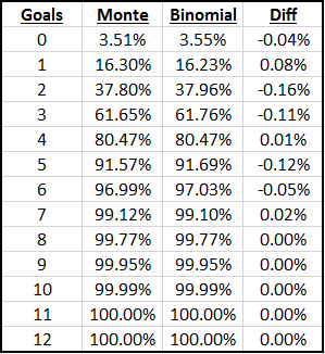
I tested to see the probability that a player scored less than a certain number of goals from a given number of shots chosen from the distribution and compared these probabilities to that of the binomial distribution with p=0.125. I used a Monte Carlo simulation with 100,000 iterations to obtain the following results. The first table shows probability of less than x goals from 1000 shots, the second of less than x goals from 25 shots.

We can see that the binomial probability runs very close to the probability based on an array of both a high and low volume of shots, never deviating more than 0.21 percentage points away.

If you have the xG values of every shot for each player, you can run Monte Carlo simulations to figure out the probability an average player would score less goals than each player. Although, as we have shown, this is well approximated by the binomial model which is much simpler and quicker to use.

Going back to our hypothetical situation we can now work out which player is a better finisher. I stuck the shots, goals, and expected goals into excel and worked out each players binomial finishing probabilities.

From this we can see that Jack Jones is the better finisher out of the two players as there’s an 81.57% chance that he’s better than an average finisher, compared to just a 58.32% chance for John Smith. This goes against the G-xG per shot model and shows an example of how players are not always being correctly ranked by the other two models.

One negative thing about this method is that it doesn’t give you the number of goals a player will add due to finishing, which the other two methods do, although this isn’t the aim of this system. The aim is to rank players based on finishing, which is what it does better than the other methods, whilst it also provides you with the probability that a player is better at finishing than average. This could potentially be beneficial in testing for repeatability, although I’ll have to check that another time.

In my next post I’m going to be using real data to see which players are the best finishers and how much this ranking system is different than the other methods. I’ll also be looking into using this method for goalkeepers in order to see which keepers are the best shot stoppers.

If you have any questions please feel free to tweet me @_peteowen