Binomial Ranking – Goalkeeper Analysis

This is probably going to be my last post on introducing the binomial probability method, I’ll try and keep it pretty short since I think I’ve explained most of the principal points already. Before reading the rest of this I’d recommend reading parts 1 and 2 if you haven’t done so already.

Since I’ve shown how the binomial method works from a finishing point of view, I’ll move on to how it can be used to asses goalkeepers’ shot stopping performance. Now, one thing that’s different for goalkeepers compared to strikers is that obviously the fewer goals the better. In order to account for this we are now trying to find out the probability that an average player would concede more goals than our player (who concedes “x” goals) given that they faced the same number and quality of shots.

To do this we can find the cumulative probability “P” that an average player would concede less than or equal to x goals (via the excel functions previously shown, or otherwise) and then take the value of “1-P” as our probability an average player would concede more than x goals.

The main difference between the binomial method for finishing and shot stopping is that the average xG for a shot ≈ 0.1, whereas the xG for a shot on target ≈ 0.3, therefore xG becomes more substantial on much fewer shots for goalkeepers. This also leads to a difference in variability between “finishing” and “shot stopping” skill, since for a binomial distribution with “n” shots and probability of scoring “p” :

Standard deviation = (n*p*(1-p)) ^0.5

Which obviously changes with different values of n and p.

This is a pretty interesting topic which I plan to delve into eventually. Looking into the difference in variability of these distributions may help with some of the problems that have been faced with finishing and shot stopping analysis. But for now let’s get back to goalkeeper analysis.

We can use some real data for visualisation. Like I said in my last post there is thankfully some openly available goalkeeper data at http://www.americansocceranalysis.com so we can use this method to analyse MLS goalkeeper performance.

I’m going to use 2014 MLS season data for analysis.

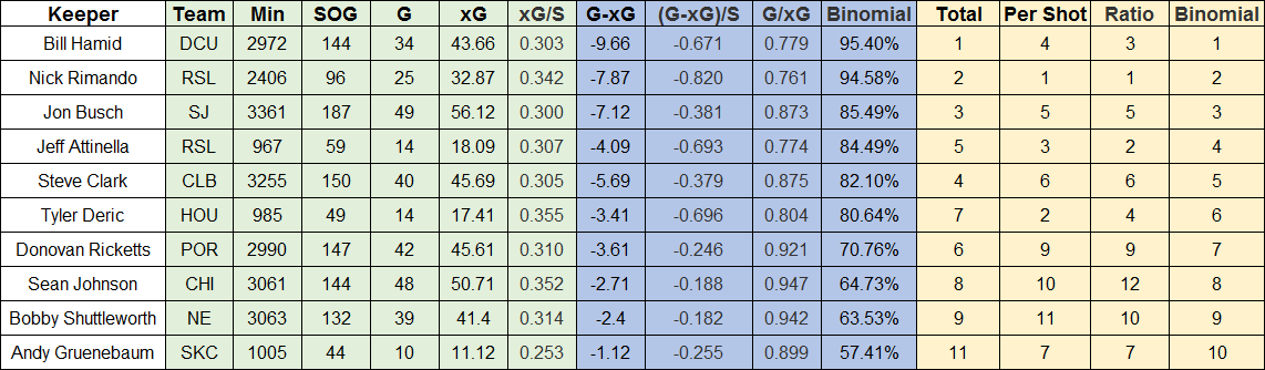
Similar to the finishing data we can notice 3 main things pretty clearly by looking at the table. Remember that for total, per shot, and ratio statistics we’re looking for low numbers since for goalkeepers the less goals the better. Notice again how:

Total – Doesn’t account for number of shots taken

Per shot – Punishes players with high number of shots [(G-xG)/S is per 10 shots]

Ratio – Punishes players with high xG values

For goalkeepers, like I stated before, it’s pretty much the same as for finishers except for the variability of the distribution, the method and reasoning are still the same. Hopefully this method can help people who are doing research into determining the value of goalkeepers, which seems to have been a pretty under researched area of analytics thus far.

If you have any questions please feel free to tweet me @_peteowen